Improve Product Review System

Improve the traditional product review system through text sentimental analysis and Natural Language Processing (NLP). By taking only the customer review comment about the product as input, I can create a sentiment detection algorithm to rate the product based on the comment. I will also include topic modeling in this project to detect the general topics of what the reviews are about.

Background and Motivation

I have an idea for this project from the situation I had when doing the thing that most college students do when they are bored: online shopping. I am a very frugal buyer myself. I spend a lot of time looking at the product description and its reviews to make sure I will not regret my purchases. Besides giant e-commerce companies (such as Amazon, Etsy, eBay, etc.), not a lot of other online retailers have anything better than a basic star and comment review system for their products. That is why, in my belief, those top-tier companies are having better customer interactions. Better customer interactions can lead to sellers improving their products and buyers, like me, have more confidence in buying the product.

Combine with a new principle I just learned that is called Principle of Least Effort (it was first articulated by the Italian philosopher Guillaume Ferrero) and the idea that businesses improve by reducing the friction that is needed for a customer to buy their product (I learned it from a book: Atomic Habits by James Clear). I want to build a review system that reduces one step needed in writing a review: rating the product. To build a system like so, I need to have the machine analyze the review comment and build a model that can predict the rating.

Since this project touch on many of the fields I am unfamiliar with, there are a couple of things that I wanted to learn out of this project that I hope will benefit my journey of becoming a better data scientist:

Scrape raw reviews from Amazon.
Learn about text and sentimental analysis.
Understand how feature engineer can give me a better outcome.
Classification algorithms and the importance of feature scaling.

Prerequisites

Python Version: 3.7.4

Packages: BeautifulSoup, requests, nltk, re, matplotlib.pyplot, seaborn, WordCloud, gensim, pandas, numpy, sklearn, itertools

Project Outline

Data collection: I build a web scrapper through BeautifulSoup and scrape an amazon product’s review. For this project, I choose a clothing item: Dickies Men’s Original 874 Work Pant. The reason for my decision is I have more experience with the product and the quantity for the review is ideal.
Text preprocessing: or data cleaning; I mostly cleaned the review texts to remove noise and make it easy for the machine to read in the data.
Exploratory Data Analysis: I analyze the target variable (“rating”) and examine its and other features' relationships. In this phase, I also perform Latent Dirichlet Allocation (LDA) topic modeling to search for topics of each rating category.
Model Building: I compare different classification algorithms (logistic regression, Naive Bayes, random forest classifier, k-nearest neighbor (KNN), and support vector machines (SVM)) and choose the one that produces the best result. The performance metric I use for my multilabel classification algorithm is the accuracy classification score that computes subset accuracy.

Data Collection

*Disclaimer: this data set is used for educational purposes.

I create a web scraper for product reviews. My first intention was to scrape 8 different variables (see table below) plus the product’s size and color. I want to see if it has any effect on determining the rating or not (such as whether such size or color has some defects). But I run into a similar issue I have with my other web scrapper: that is I cannot make the function see null value as n/a and it will just skip over. So I decided to leave those two variables out of the data set. Although I want to scrape all 9,208 reviews it has, Amazon only allows me to access only 5,000 of the reviews. Hence, my data scrapped CSV consists of 8 variables and 5,000 records.

Variables	Description
customer_id	the unique ID of each customer
customer_name	name of the customer
rating	customer’s rating of the product (1-5)
review_date	review’s posted date
review_loc	customer’s location (only take reviews from the United States)
verified_purchase	customer’s product purchased verification
review_head	review’s title
review_body	the main part of the review

Text Preprocessing

By glancing at the data set: according to figure 1, only one of our data is numerical (“rating”) and the rest is categorical. Another important element is to determine whether there is any null value. Luckily for me, there is none.

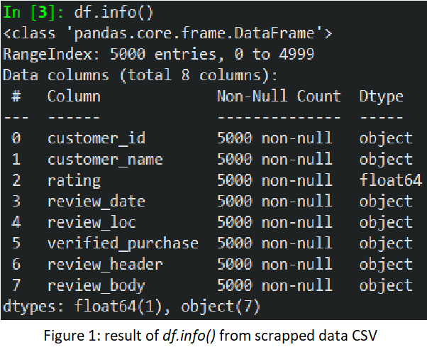
I combine both the review’s header and body for easier analysis later on. And since both “verified_purchase” and “review_loc” only have one unique value for each variable, I remove them from the data set because it will not give us any information.
Generalize “review_date”: To see the relationship between “rating” and “review_date”, I need to group the individual date for a more compact and reasonable graph later on. I want to group them by quarters at first, but I find that I need to compact it even more so I end up doing it by years instead.
Then, I create a function (“clean_text”) to perform text preprocessing to the review texts. I implement the following steps: convert text to lowercase, replace contractions with their longer forms, remove punctuations and numbers, tokenization (a process of splitting strings into tokens), remove stop words, lemmatization(return a word to its common base root while takes into consideration the morphological analysis of the words), only get word that has more than one character. Since there will be some short reviews that end up with empty values after the text is cleaned, I remove them from the data set.
I will do a bit of feature engineering and use VADER Sentiment (SentimentIntensityAnalyzer) as a sentiment analysis tool to analyze the emotion of the review text. This tool is very good at not only determine whether a string of text is positive or negative, but it also gives the string a sentiment intensity score. Since the score is ranged from [-1,1], I label the score as follows:
- score >= 0.6: 5
- 0.6 > score >= 0.2: 4
- 0.2 > score >= -0.2: 3
- -0.2 > score >= -0.4: 2
- -1 >= score: 1
Lastly, I will add two more features by determining the string character’s length and word count.

EDA

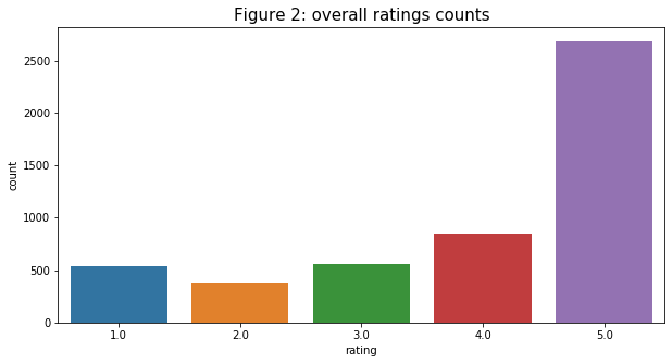
Univariate analysis on target variable (“rating”): I first look at the count of each rating to see if there is an imbalance. From the bar chart in figure 2, ratings from “1” - “4” are in a close range (from 400 - 750 counts range), but the rating of “5” has over 2600 counts. Although it is quite substantial, in terms of business, there are many more customers that are very satisfied with the product than those that are not. We can say that, overall, customers are happy with their purchases.

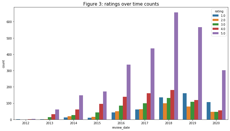
Multivariate analysis on target variable (“rating”): next I add time as another element to the analysis. I am wondering whether time has any effect on the customers' rating: maybe the product was bad and people gave negative feedback then the manufacturer improved it and people liked it more or vice versa? Based on the figure below, it turned out that the trend is quite the same. From 2013 to 2017, the rating count is ranked that “1” has the lowest count, and the higher the rating the higher the count. It is not until 2028 to 2020 that the count for “1” increases in terms of count and proportion of the rating for the year and is ranked as the second-highest count rank. We do not have enough information to conclude that, in general, customers are not liking the product anymore. But these are very good data for the manufacturer to start taking into consideration.

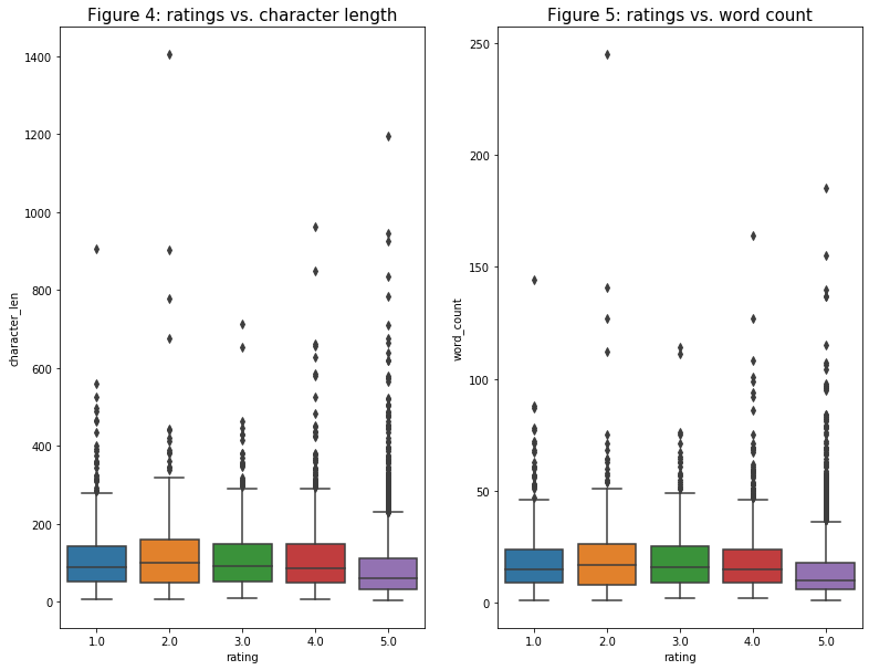
Next on the list are “rating” vs. “character_len” and “rating” vs. “word_count”: because both box plots have very similar trends so I will analyze them as one. My initial assumption was that there would be a semi-clear trend of the higher the rating, the fewer words or character length the review has. Although there would be outliers (say a customer loves the product and ending up writing paragraphs about it), my assumption is based on the fact that customer is more likely to criticize more when they are dissatisfied with the purchase. Two graphs below prove my assumption, but the trend is not as clear as I imagine it would be: the “5” rating’s count range and the median is smaller than the others, but the differences are not too significant. Maybe the result would be better if I graph these variables before cleaning the review text.

Figure 4 & 5

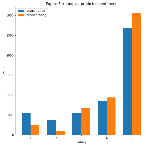
My last multivariate analysis is to see how accurate is the VADER Sentiment in column “predict_sentiment” by comparing its and the “rating” count. Based on the figure below, it does not predict as well as I would hope for. From “3” to “5” rating, the differences between the two counts are not as big of a gap. But it does pretty badly when trying to predict the sentiment of the “1” and “2” ratings. I can conclude that the VADER Sentiment might be over-rating the sentiment, so I need to expect to see many reviews where they are rated negatively but the “predicted_sentiment” variable incorrectly states that it is positive.

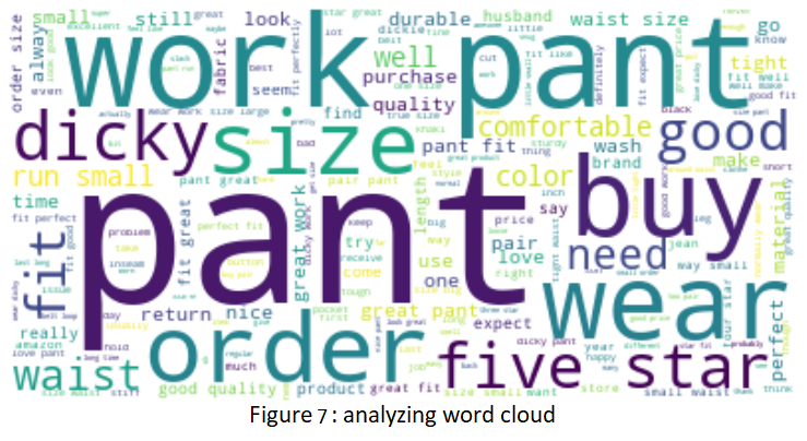
After analyzing the variables, I want to have a closer look at the cleaned review text itself. I create a word cloud of all the review text for this product in figure 6. This has a very good representation of what words are being repeated the most by having it in different font sizes (the bigger the fonts, the higher the counts). Just by looking at the picture itself, besides the obvious, here are some observations:
- I can see many text from “5” star ratings: “five star”, “perfect”, “buy”, “great work”, etc.
- I can also get a sense of what most of the reviews are about: “size”, “quality”, “durable”, “fit”.
- Negative review’s texts are also present in the word cloud: “run small”, “waist size”, “tight”, “return”, etc.

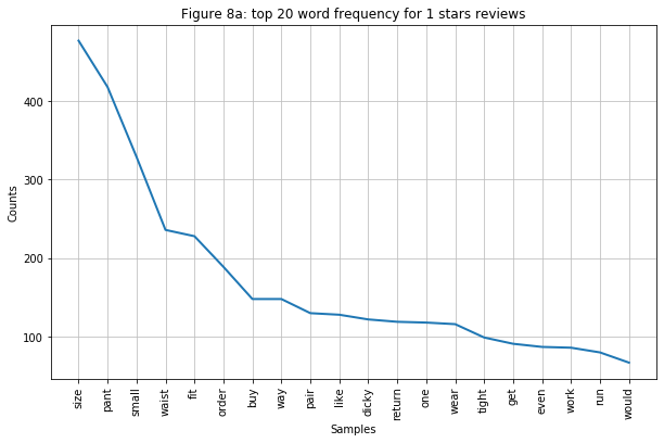
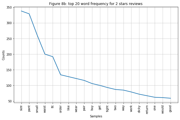
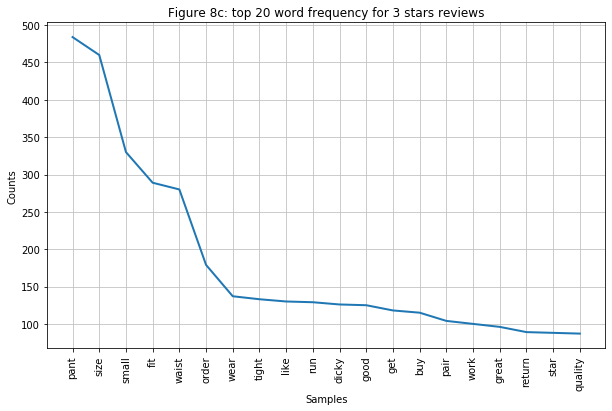
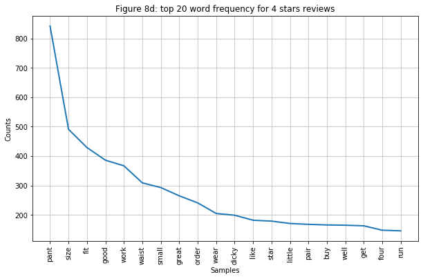
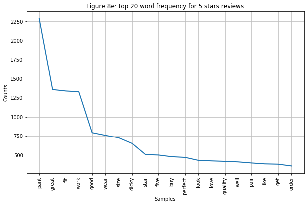
Word cloud might be a great tool to have a general understanding of the text, but I can analyze it better if I look specifically at the word frequency of each rating. Below are frequency graphs of the top 20 words from the five ratings. Here are some observations:
- Figure 7a-7c: I grouped these three graphs because they have a similar trend. Just by looking at the top 5 words with the highest frequency (“size”, “pant”, “small”, “waist”, “fit”), I can already see that customers are not satisfied with the product is not happy about sizing the most. It is not a surprise to see many people would return the product because the word “return” is also in the graph.
- Figure 7d: this is where we see the turning point the clearest: this graph has more positive words ranked top of the graph. Interestingly, the word “small” is still present in the top 10.
- Figure 7e: this graph is filled with only neutral to positive words. But also interesting to note, although reviews do seem to compliment the fitting of the product, they seem to be more positive than previous ratings.

Figure 8a Figure 8b Figure 8c Figure 8d Figure 8e

For my final analysis, I implement the Latent Dirichlet Allocation (LDA) topic modeling. Although this step may seem repetitive, because the outcome might just be similar to what I have analyzed, I want to see how accurate is this unsupervised learning approach in identifying topics that are being talked about in the reviews' text. It turns out that LDA topic modeling identifies the topics quite well. Below are the result and five examples from each rating:
- 1-3 stars reviews: consist of mostly “size”, “pant”, “small”, “waist”, and “fit” words. They indicate that the pants are too small around the waist for those unhappy customers.
- 4-5 stars reviews: consist of “pant”, “size”, “fit”, “good”, and “work”. They indicate that the pant has a good fit. “work” here might also means that it is great for them to do their work in since this is a workwear type of pants.

Figure 9a Figure 9b

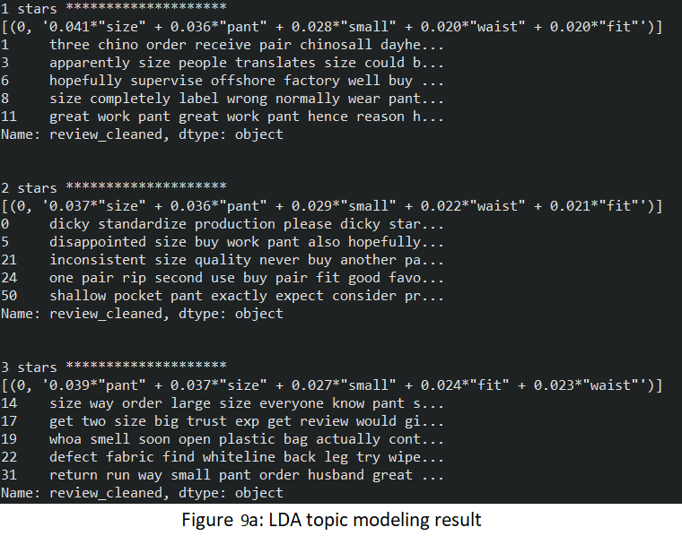
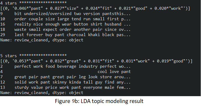
This makes me wonder about the product sizing being polarized. Although different people have different shapes and sizes might be a good guess, but it does not align with the number of dissatisfied reviews. So, my assumption has to do with different sizes of the product that might cause these criticisms: that is some product sizes might be scaled disproportionately.

Model Building

Perform vectorization on review texts: the process of converting words into numbers so that the machine can understand. For this project, I use Term Frequency-Inverse Document Frequency model (TFIDF) vectorizer + ngrams (bi-gram) technique. I have tried it with different ngrams (monogram, bi-gram, tri-gram) but it seems that bi-gram help to produce the best result.
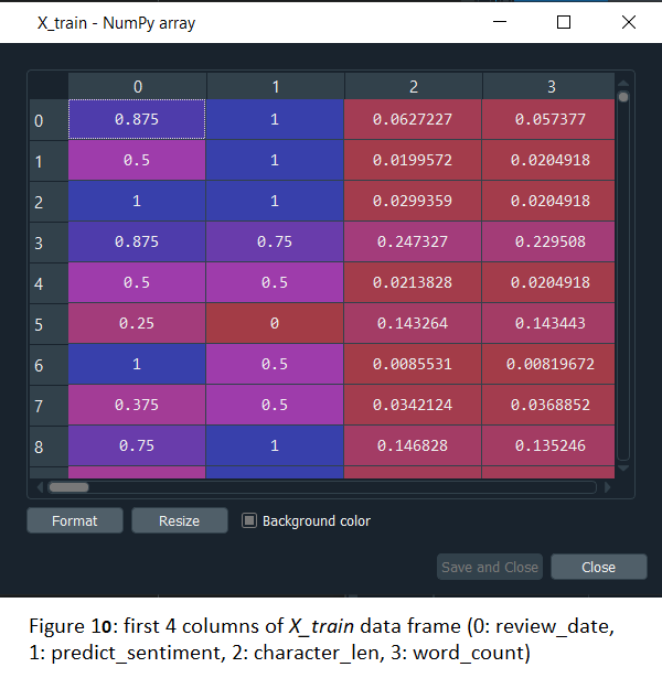
After removing unnecessary columns (“customer_id”, “customer_name”, “review_header”, “review_body”, “review_txt”, “review_cleaned”, I split the data to training (80%) and testing (20%) sets in a stratify fashion: stratas are the different ratings. The reason for this there is a lot more “5” stars rating compares to others. By splitting it in stratify fashion, I can eliminate the bias of having an over-whelmed majority of that rating.
Because the data has many different ranges of value (such as character_len and those text vectorization columns), I rescale those values into a 0 to 1 range using the function MinMaxScaler. This helps the model produce a more accurate result.

The first model I apply for this data set is the Logistic Regression. Although the model is known more for its binary classification, not quite what I want to predict (which is 5 different ratings), I want to apply it in this project to see how it does compare to other more advanced ones. By having the “multi_class” parameter as “multinomial”(which uses the cross-entropy loss), I can apply it for my multiclass case. I also test it with different “C” (inverse of regularization strength) of values 0.01, 0.05, 0.25, 0.5, 1 to see which one gives the highest accuracy. Though this is a more simple model compare to the rest, so I expected the accuracy will not be as high.

for x in [0.01, 0.05, 0.25, 0.5, 1]:
    log_reg = LogisticRegression(C=x, solver='lbfgs', multi_class='multinomial', random_state=1).fit(X_train, y_train)
    print ("Logistics regression accuracy (tfidf) for ", x, ":", accuracy_score(y_train, log_reg.predict(X_train)))

log_reg = LogisticRegression(C=1, solver='lbfgs', multi_class='multinomial', random_state=1).fit(X_train, y_train)
print ("Logistics regression accuracy (tfidf) for C=1:", accuracy_score(y_train, log_reg.predict(X_train)))

Out[2]: 0.9872372372372372

I apply the Gaussian Naive Bayes Classifier, a variant of Naive Bayes, for the next model comparison. Since this algorithm has a different approach in building up a simple model (by assuming data is described by a normal distribution), I am curious to see how this simple supervised learning algorithms perform compares to others.

naive_bayes = GaussianNB().fit(X_train, y_train)
print ("Naive Bayes accuracy: ", accuracy_score(y_train, naive_bayes.predict(X_train)))

Out[4]: 0.9204204204204204

Another supervised learning algorithm is the random forest classifier. But unlike the two algorithms above, it uses decision trees combination and voting mechanisms to perform its prediction. Because the random forest classifier is not biased and more stable when get fed with new data (opposite from Logistics Regression), I want to test out this algorithm after being concerned the algorithms above are both overfitted by producing such high accuracy scores (above 90%).

randomfor_reg = RandomForestClassifier(n_estimators=1000, max_depth=10, random_state=0).fit(X_train, y_train)
print ("Random forest classifier accuracy: ", accuracy_score(y_train, randomfor_reg.predict(X_train)))

Out[6]: 0.5367867867867868

An algorithm that uses a similarity measure of data points to perform classification is K-Nearest Neighbors Classification. This is a good algorithm to use if the data is not linearly separable.

k_neighbor = KNeighborsClassifier(n_neighbors=15).fit(X_train, y_train)
print ("K-Nearest neighbor accuracy: ", accuracy_score(y_train, k_neighbor.predict(X_train)))

Out[8]: 0.5535535535535535

Last but not least, I use the Support vector machines (SVMs) as the last model to perform classification and compare the result. Because SVMs have been reported to work better for text classification and it is very effective in high dimensional spaces, I expect this to return relatively higher accuracy compares to the rest.

supportvector = svm.SVC(decision_function_shape="ovo", random_state=1).fit(X_train, y_train)
print ("SVM accuracy: ", accuracy_score(y_train, supportvector.predict(X_train)))

Out[10]: 0.9109109109109109

Overall Model Performance

The accuracy scores of the training data set from the five models above surprise me. Specifically, the three models that give the highest scores are Logistic Regression (98.72%), Gaussian Naive Bayes Classifier (92.04%), and Support vector machines (91.09%). The two worst-performing models are the random forest classifier (53.68%) and K-Nearest Neighbors Classification (55.35%). It is also interesting to note there are two clusters of accuracy scores produced by the models above.

My initial thought was that the top performance models are overfitted. Although I did apply many crucial text pre-processing techniques, any accuracy scores that are above 90% when dealing with real-world data is a bit too high. I would not be concerned if the two most simple classifiers (Logistic and Gaussian Naive Bayes) would be overfitted, but SVMs should not be.

Moving on to the cluster of lower score models. Although the scores are a lot lower than the other cluster (at least 36% score difference), not only they are above the 50% mark, these models do not have the overfitting problem (hence the reason I included them for this project).

The next step is to implement these models to the test data set to see how well they can predict the ratings based on customers reviews:

log_reg_test = log_reg.predict(X_test)
naive_bayes_test = naive_bayes.predict(X_test)
randomfor_reg_test = randomfor_reg.predict(X_test)
k_neighbor_test = k_neighbor.predict(X_test)
supportvector_test = supportvector.predict(X_test)

print('Log regression: ', accuracy_score(y_test, log_reg_test))
print('Naive Bayes: ', accuracy_score(y_test, naive_bayes_test))
print('Random forest regression: ', accuracy_score(y_test, randomfor_reg_test))
print('K-nearest neighbor: ', accuracy_score(y_test, k_neighbor_test))
print('Support vector machines: ', accuracy_score(y_test, supportvector_test))

Log regression:  0.6396396396396397
Naive Bayes:  0.4244244244244244
Random forest regression:  0.5375375375375375
K-nearest neighbor:  0.5545545545545546
Support vector machines:  0.6046046046046046

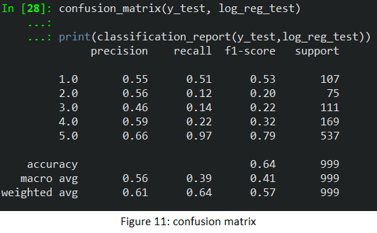
As expected, while there is not a major difference between test data accuracy scores and training data accuracy scores for the lower score models' cluster, the higher score models' cluster test data accuracy scores drop (might due to the model simplicity, Naive Bayes becomes the worst performing model). By being the best performing model in the train data, Log regression is also the best model in the test data with a 63.96% accuracy score.

In the figure below, I apply a confusion matrix to the multi-class classification model. Besides the chosen metric (accuracy score), there are three more to be considered: precision, recall, and f1-score. Precision answers the question: what is the proportion of all predicted positive being truly positive? Recall answers the question: what proportion of actual positives is correctly classified? In other words, precision emphasizes the false positive, and recall emphasizes the false negative. Because false positive or false negative outcome does not have much of a difference, let’s look at the f1-score instead. F1-score is a good metric for my case because it is the balance between precision and recall. Figure 11 shows that the macro average of the f1-score is 0.41 and the weighted average of the f1-score is 0.57.

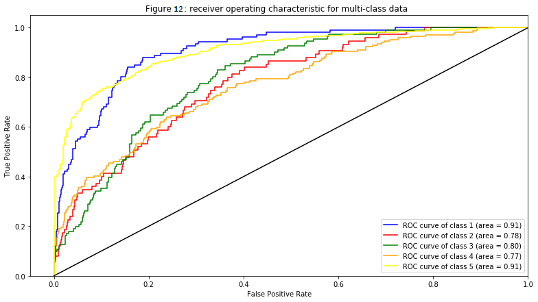
Lastly, I plot the area under the curve (AUC)- receiver operating characteristic (ROC) curve. This plot tells us, specifically, how well my model can distinguish the classes (ratings) by showing the trade-off of true positive rate and false-positive rate for different threshold settings of the underlying model. Generally, if the curve is above the diagonal line (chance level) and the area is above 0.5, it can be considered a good ROC curve.

Conclusion

Based on the accuracy score being almost 64%, it is safe to say that the Log regression model predicts the rating based on the customer’s review quite accurately. Since I also consider other metrics, I do need to keep in mind that f1-scores are quite low (especially the macro average of the f1-score being below 0.5). Taking a look at the AUC-ROC curve, by having all AUC values above 0.75, proves that this model can also distinguish the different ratings very well. In conclusion, I have reached my goal for this project by not only making the model works but also make it produce a great result.

I believe that with more data from other ratings (since “5” stars rating takes a big proportion of the entire data set), the model’s accuracy scores will be improved. Because I have a large enough sample size, I could have applied k-fold validation to eliminate the overfitting problem while predicting the train data set.

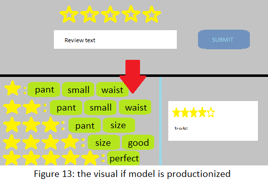
If I was to continue this project, I would apply some front-end works by productionize the model. I want to make it predicts the rating I want to give to a product based on the sentiment of my review text after I hit the submit (submit the review) button. After that, it will analyze all the reviews per rating and pick out the keywords of each rating. This helps the customer to see what are the most commonly discussed topic from each of the ratings. If I can apply this system to an online store, it will eliminate a step that requires a customer to write a review and help them to get a glance at what others are saying about the product before buying. Hence better customer experience and interaction.

Code

This project’s codes can be viewed at this GitHub’s repository.

Update! (06/10/21)

I had successfully deployed the machine learning model using Heroku and Streamlit! Check out this website for the application: https://amazon-product-review-star.herokuapp.com/. Also, you can check out my “Improve_Review_System_Deploy” repository for the code and data files.