Stock Price Prediction

Predicting HSBC Bank stock prices to make better buying/ selling decisions using an artificial recurrent neural network (RNN) architecture: Long short-term memory (LSTM). In addition to using past prices for prediction, I applied some stock technical analysis that I learned to see if it can outperform the deep learning model.

Background and Motivation

“The greatest risks are never the ones you can see and measure, but the ones you can’t see and therefore can never measure. The ones that seem so far outside the boundary of normal probability that you can’t imagine they could happen in your lifetime–even though, of course, they do happen, more often than you care to realize” - Joe Nocera

Recently, I took an interest in learning about the stock market and how day trading works. That was very odd of me considering countless times I heard people say that you will end up losing money when trading the market. But funny how a random guy on YouTube convinced me by saying something along the line of losing trades and losing trades but risk management are two different things, one will make you lose money and the other will make you a better trader. Then, the YouTube channel that I used to learn about the topic and bet my future financial decision on is called Real Life Trading by the guy mentioned above, Jerremy Alexandar Newsome. Although the channel seems gimmicky at first, Jerremy did an excellent job of simplifying how the market and all of its basics (at least for the introduction course I am taking). Getting further into the material, I started to learn about different indicators that predict the stock movement and the meaning of those indicators. I was surprised to hear that, as a trader using mostly technical analysis to trade stock as Jerremy himself, those indicators that he taught me are things he considered the most when making his stock decisions.

As an aspiring data scientist, I saw that stock technical analysis is simply using past data to predict future outcomes. Since many of the supervised learning algorithms function the same way, I decided to see if I could apply one of the algorithms to a history of stock prices and predict what the future prices will be. I chose to apply the Long short-term memory (LSTM) algorithm to predict the stock prices. My goal for this project is to see how accurately can a machine predict the stock market and therefore answers the question of whether I can depend on the prediction to make my trading decision. Here are two things I would like to learn our of this project:

Create technical analysis indicators on Python
Learn how an artificial recurrent neural network (RNN), specifically LSTM, works

Disclaimer: I am in no way shape or form an expert in trading the stock market and would not recommend anyone to use this model to base their trading/investing decision.

Prerequisites

Python Version: 3.7.4

TensorFlow Version: 1.14.0

Packages: numpy, yfinance, mplfinance, random, pandas, matplotlib, seaborn, sklearn, tensorflow, datetime.

Project Outline

Data Wrangling: I got stock price data of HSBC bank from a Python library called yfinance and created 18 additional indicators that acted as variables based on the stock prices. All candlestick-related knowledge that I used is based on Jerremy’s ebook: “EVERYTHING YOU NEED TO KNOW ABOUT CANDLESTICKS”.
Exploratory Data Analysis (EDA): plotting three different plots showing: long-term trend, short-term trend, and current trend. I also created a candlestick chart using mplfinance library. Then, I implemented a simple trading plan only using moving averages and plotted it.
Model Building: first, I normalized the data and split them into train and test data sets. Then, I built a stacked LSTM model and plot the prediction. Lastly, I did the same step as previously but try to predict the prices for the next 30 days and plot them. The performance metric I used for my model is the root mean square error (RMSE).

Data Wrangling

Through yfinance library, I got stock prices of ticker “HSBC” from May 12th, 1995 to July 27th, 2020.

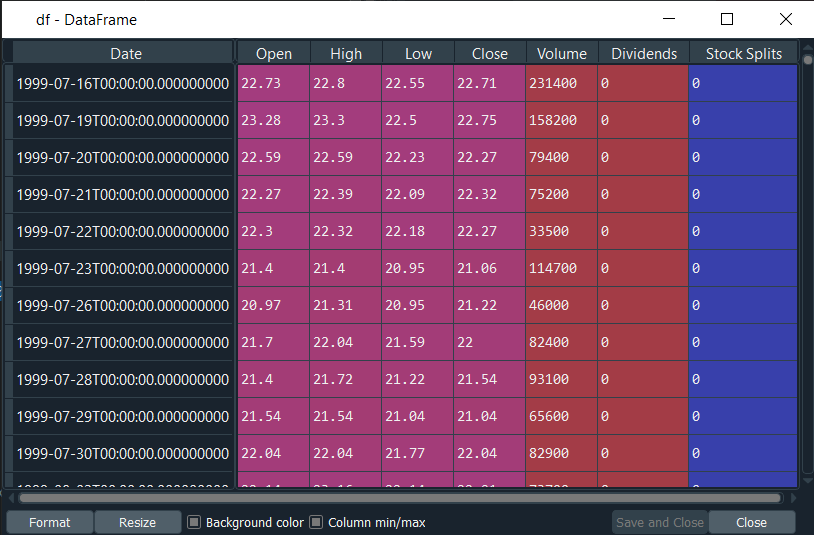
I turned the data frame index to a new column “Date”.
To prepare for candlesticks visualization, I created a function (“candle_stick”) with the mplfinance library embedded. This function will return a maximum of two candlestick plots of the candlestick’s pattern. For easy use, I made it so whatever the candlestick or pattern will be the candle(s) in the middle of the graph. Along with it will be ten extra days of data before and after the candlestick/ pattern happened.
I created a list to get the body sizes of every candle (the absolute value of the difference between the open and close price of the day). This became handy later on when I need to find the mean of body size.

Below are formulas that I used to create different candlesticks/patterns and their plots:

Please note that, in some way, candlestick can be seen as a form of art: meaning that there are no set-in-stone functions that define every candlestick/pattern. Functions I used for this project are very simple and straightforward.

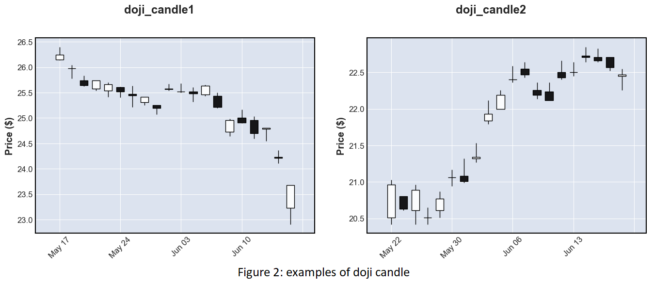
Doji candle: a candle without a body. Function: absolute value or the difference between the open and close price of the day equals zero.

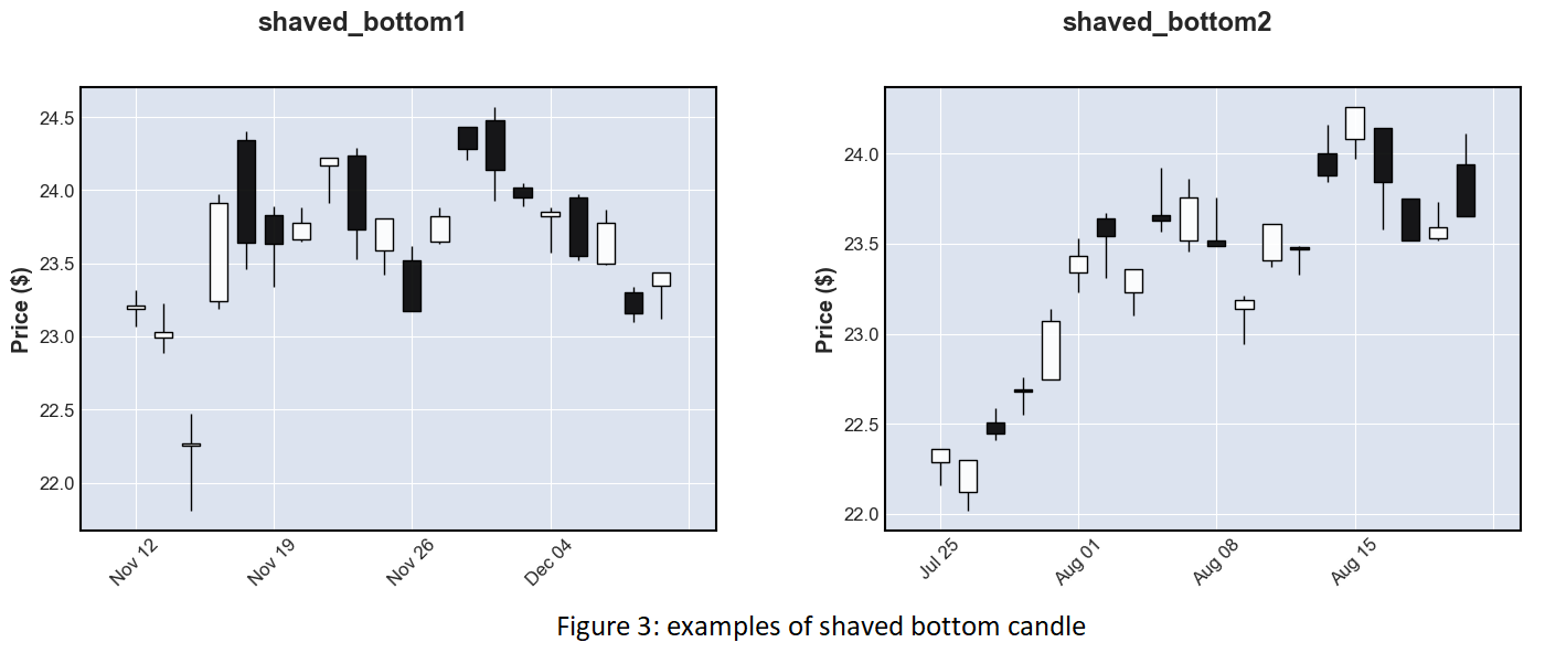
Shaved bottom: A candle without a lower wick. Function: the closing price equals the low price of the day.

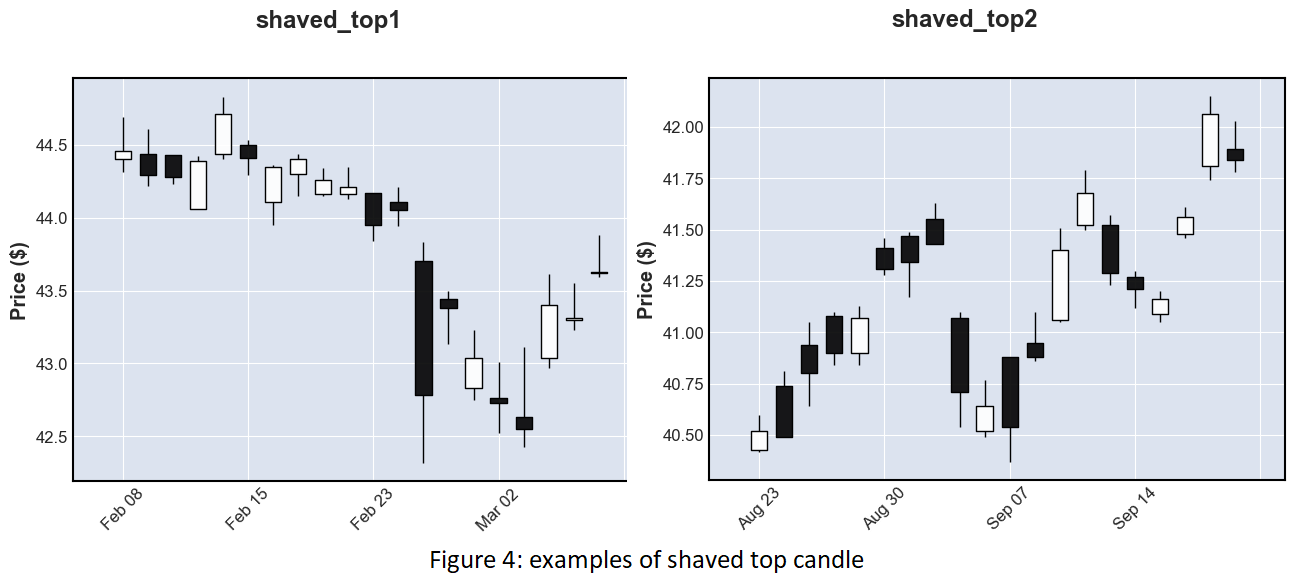
Shaved top: A candle without an upper wick. Function: the open price equals the high price of the day.

Bullish marubozu candle: white shaved bottom and top candle with a size much larger than the average candle. Function: the difference between close and open price need to be positive and bigger than the average candle by 1.5 times, high equals close, and low equals open price of the day.

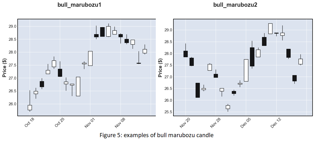
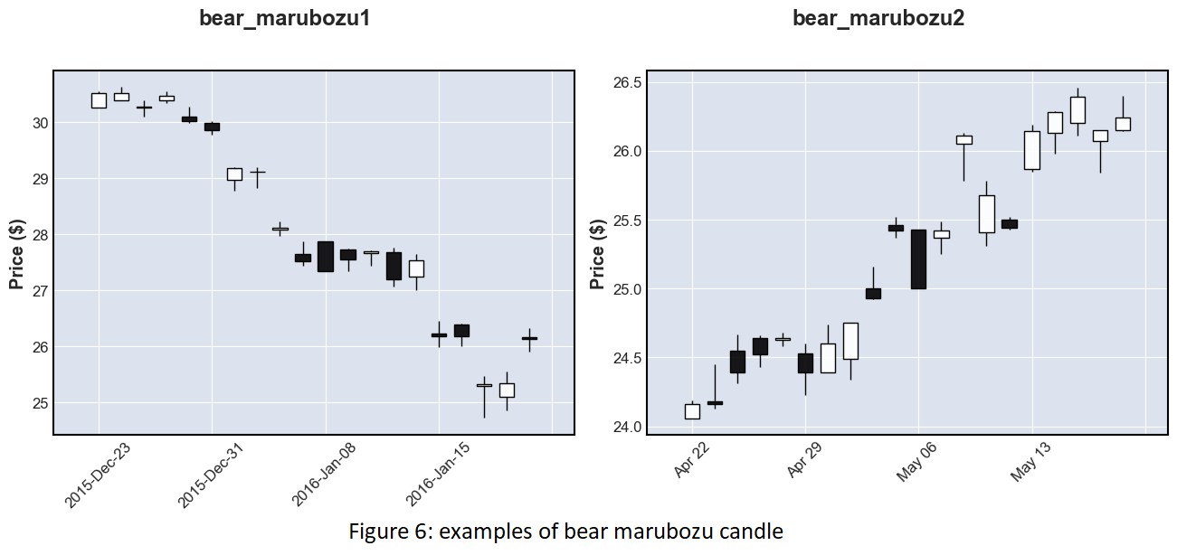
Bearish marubozu candle: black candle version of bullish marubozu candle. Function: the difference between close and open price need to be negative and bigger than the average candle by 1.5 times, high equals open, and low equals close price of the day.

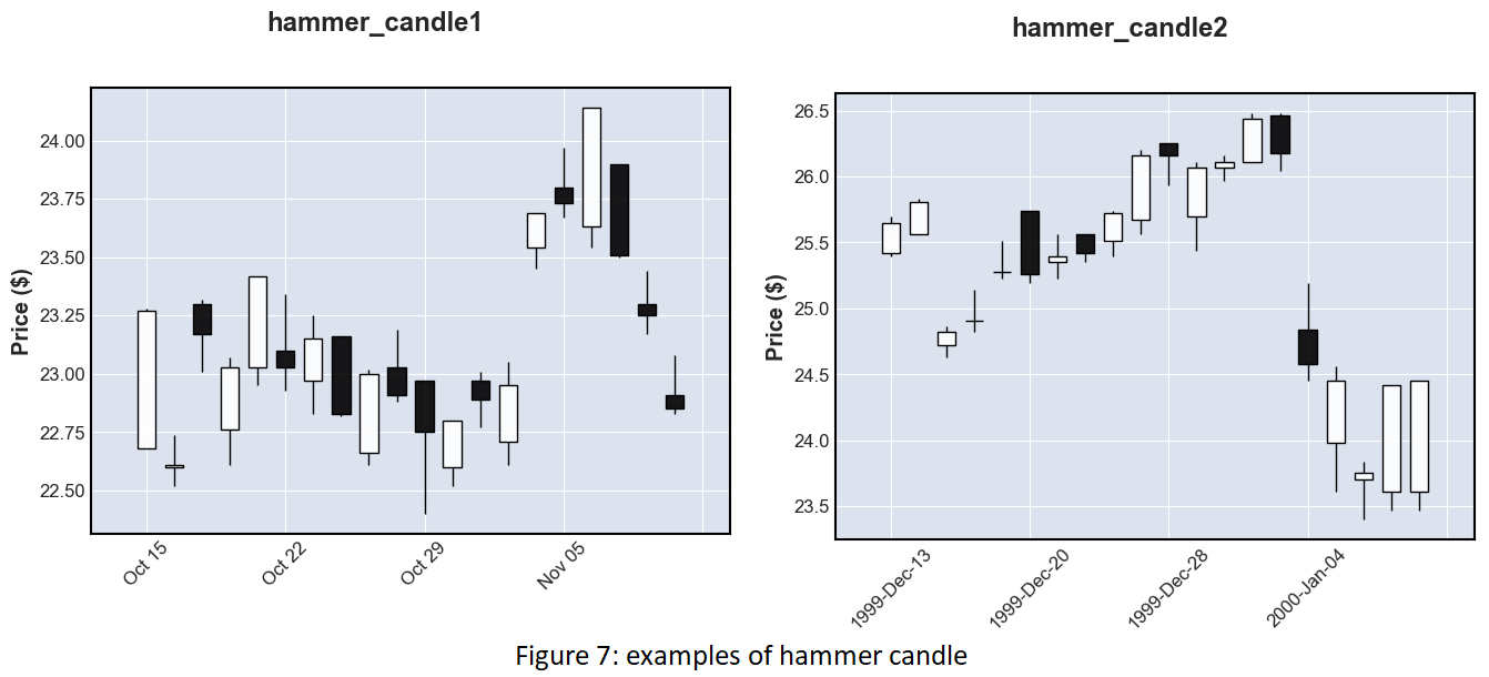
Hammer candle: the lower wick of the candle should be about two times the size of the candle body; the candle still has a body but no upper wick. Function: high equals the open price of the day, the difference of the close and low price is bigger than the difference between close and open prices multiplies by 1.5 times.

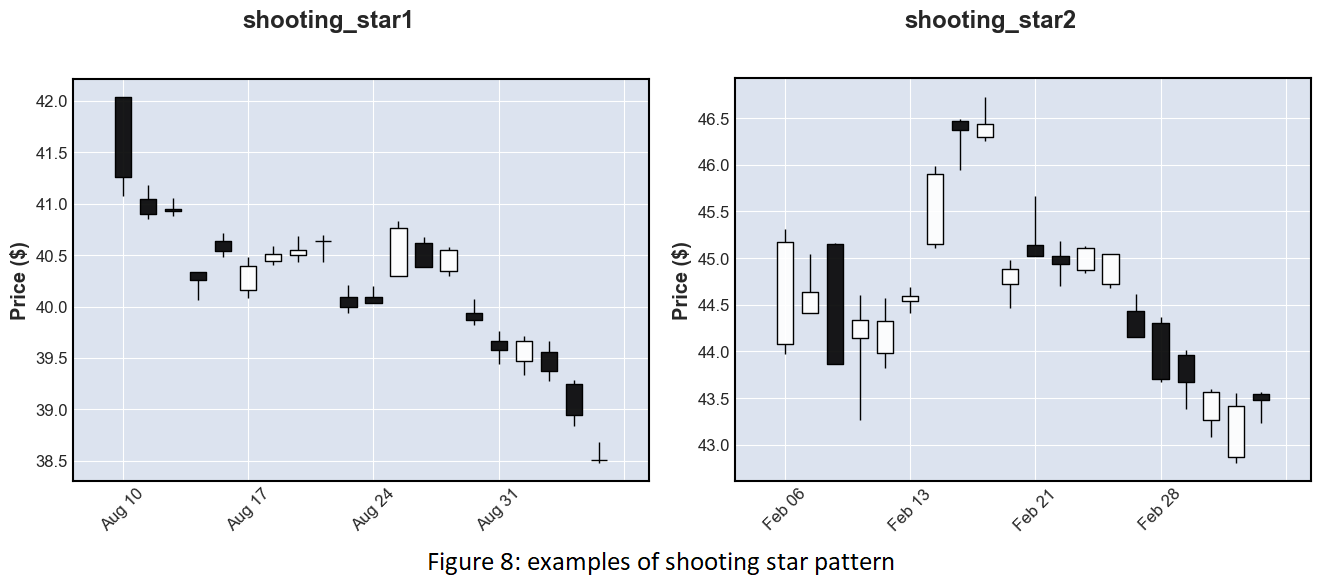
Shooting star candle: the inverted hammer candle. Function: low equals the close price of the day, the difference between the high and open price is bigger than the absolute value of the difference between open and close price multiplied by 1.5 times.

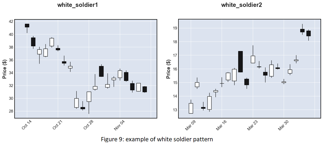
One white soldier pattern: the open of a white candle has to be above the close of the previous day’s black candle and The close of the white candle has to be above the open of the previous day’s candle. Function: the difference between close and open price needs to be positive and bigger than the average candle by 1.5 times, open of the candle needs to be bigger than the close price of the previous candle, and close of the candle needs to be bigger than the open price of the previous candle.

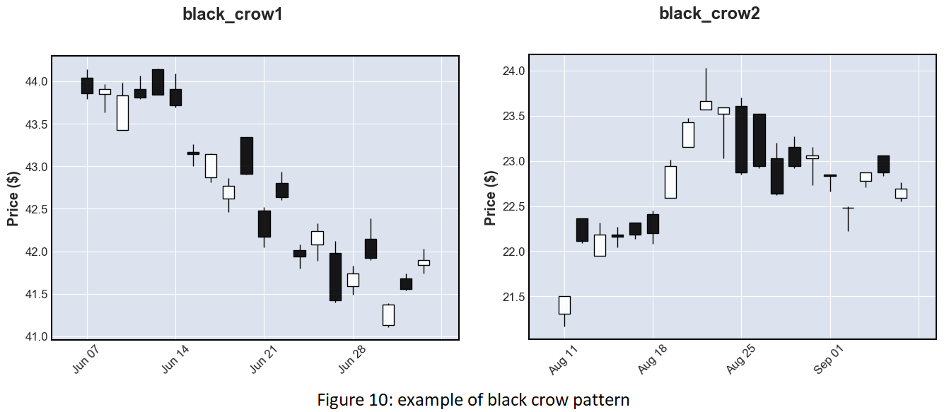
One black crow: the open of a black candle has to be below the close of the previous day and the close of the black candle has to be below the open of the previous day. Function: the difference between close and open price needs to be negative and its absolute value needs to be bigger than the average candle by 1.5 times, open of the candle needs to be smaller than the close price of the previous candle and close of the candle needs to be smaller than the open price of the previous candle.

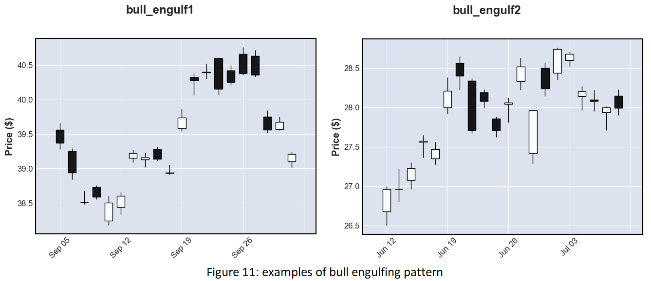
Bullish engulfing pattern: the open of a white candle must be below the low of the previous black candle and the close of the white candle must be above the high of the previous candle. Function: the difference between close and open price needs to be positive, the open is smaller than the low price of the previous candle, the close is bigger than the high price of the previous candle, and the difference of close and open price of the previous day needs to be negative.

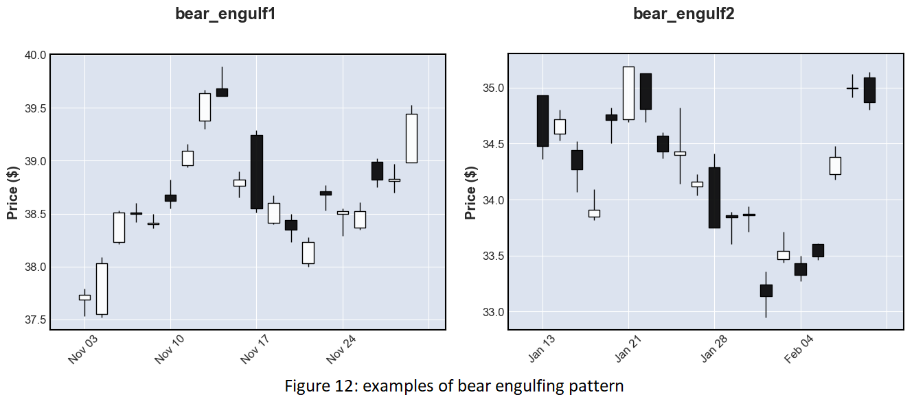
Bearish engulfing pattern: the open of a black candle must be above the high of the previous white candle and the close of the black candle must be below the low of the previous candle. Function: the difference between close and open price needs to be negative, the open is bigger than the low price of the previous candle, the close is smaller than the high price of the previous candle, and the difference of close and open price of the previous day needs to be positive.

Tweezer top: a white candle follows by a black one with an equally high price. Function: high equals the high price of the previous day, the difference of close and open price needs to be negative and the difference of close and open price of previous day candle needs to be positive.

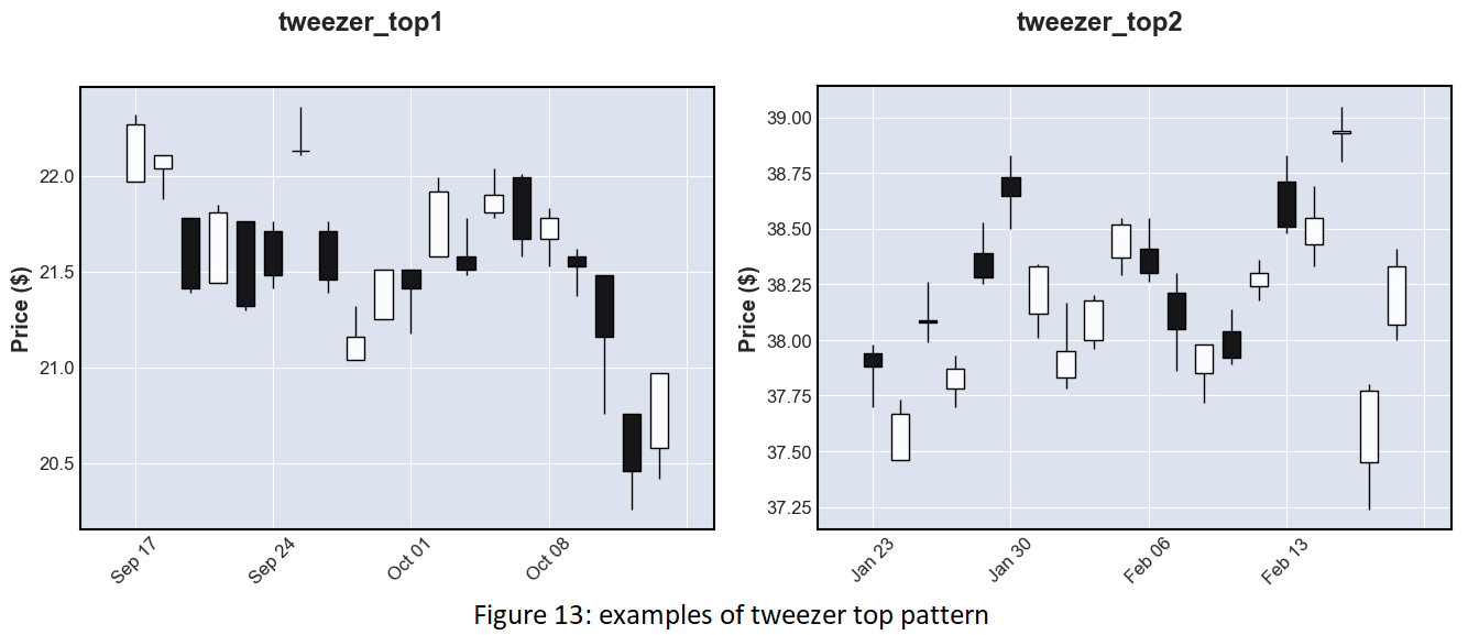
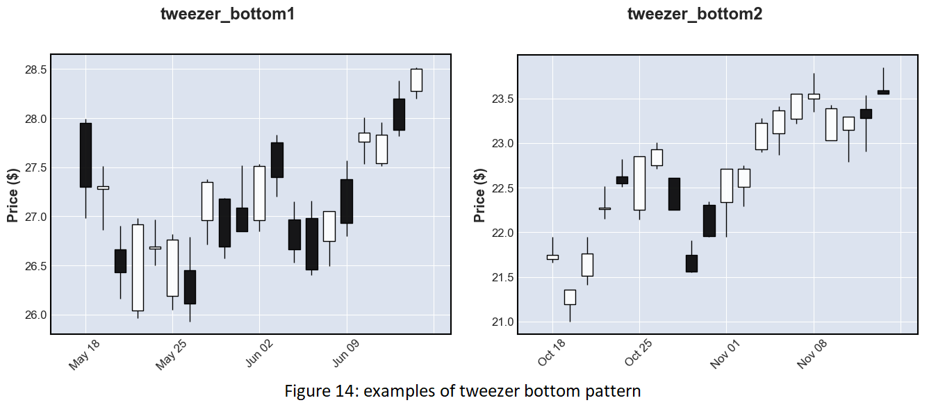
Tweezer bottom: a white candle follows by a black one with an equally high price. Function: high equals the high price of the previous day, the difference of close and open price needs to be positive and the difference of close and open price of previous day candle needs to be negative.

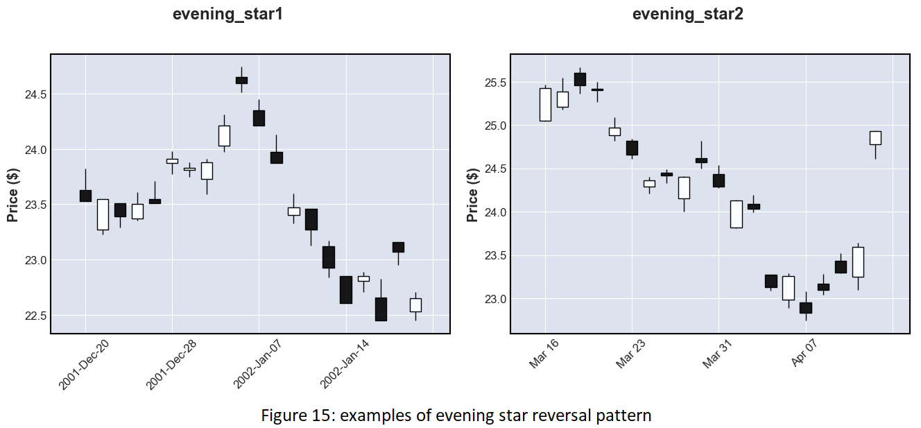
Evening star reversal pattern: a white candle follows by two black candles. The low price of the previous day’s candle is bigger than the high of the second previous day’s candle. The high price is smaller than the open of the previous day’s candle. Function: the difference of close and open of the second previous day candle needs to be positive, for the previous and current day needs to be negative. The low of the previous day is smaller than the high of the second previous, high is smaller than the open price of the previous day.

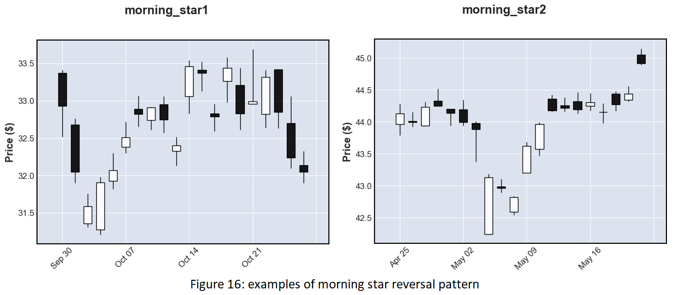
Morning star reversal pattern: a black candle follows by two white candles. The close price of the previous day’s candle is smaller than the low of the second previous day’s candle. The high price of the previous day is smaller than the open price. Function: the difference of close and open of the second previous day candle needs to be negative, for the previous and current day needs to be positive. Close of the previous day is smaller than low of second previous, high of the previous day is smaller than the open price.

Next, I created two different exponential moving averages: the 20 exponential moving average (moves slower) and the 50 exponential moving average (moves faster).
The last variable that I included in the data frame is “percent_change”, which calculates the percentage of change of the closing price.

EDA

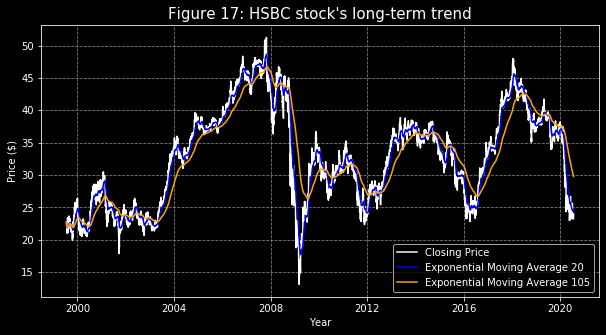
To determine whether the stock is good to buy, the first thing I needed to do is to look at the overall trend (long-term) of the stock price history. The line graph below shows that the overall trend of this stock is sideways, which is not bad because at least it is not going down. The stock had its highest price in 2007 at around $55 and fell rapidly at the end of 2008 to around $12 (probably due to the Great Recession that happened in that period). From there, its pattern is quite predictable. Based on the graph, assume that there is not an event that causes a severe change to the market (like the current pandemic), the stock is very likely to bounce back up to the $38 price mark. I would be very interested in this particular stock if I am a trader compare to an investor.

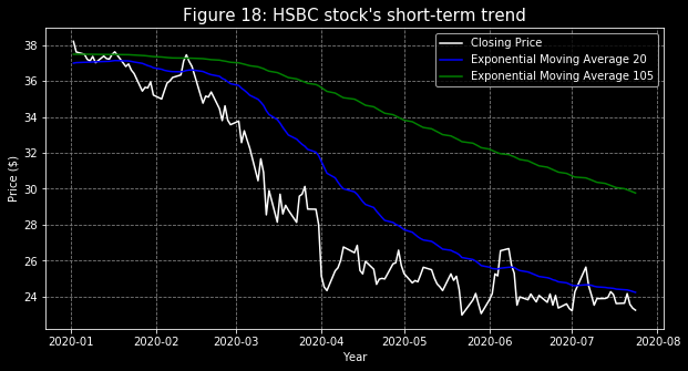
Next, we will look at a closer picture: a short-term trend. I defined the short-term here as data starting from January 2nd, 2020 to July 27th, 2020. The line graph below shows that there is a downward trend (or a bearish trend), though it did platten out at the end. Many traders will look at this graph and go “Welp, that’s it for this stock.” But since I already looked at the bigger picture (long-term trend), I knew with a certain degree of confidence what the stock is going to do next. In another word, I will act differently from those traders. If I predicted the stock will go back up, this is a perfect time to buy the stock when the price is low. If the plan works out, the return will be incredible.

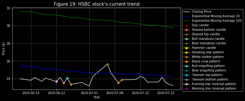
Since I knew what I should do with the stock, then the next challenge is to figure out where to enter the trade. Based on the course I took from Jerremy, I need to look for an indicator. A specific candlestick/ pattern that indicates the stock will go up (or go bullish). I created even a smaller picture, a line graph of stock price history for the last 30 days, to look out for details. Since I couldn’t add markers to the candlestick graph, I labeled it in the line graph below with a different colors marker to spot the special candlestick/ pattern. In the line graph, there were a couple of candlesticks/ patterns appeared in the last 30 days: shaved bottom candles, white soldier pattern, bull engulfing pattern, and evening star reversal pattern. Besides the fact that those candlesticks/patterns did not affect the trend much, there wasn’t any indicator coming up in the past week, I should be patient and wait for now.

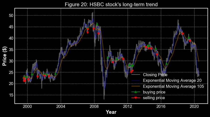
This last step is additional visualization that can be improved later on: I created a simple trading plan and graph it on the line graph. This plan only involves two exponential moving averages: if the 20 exponential moving average is above the 50, buy the stock; sell the stock if it is reversed. I used the interceptions of those two lines as indicators of where I should buy/ sell the stock.

Model Building

For this part of my project, I wanted to give credit to Krish Natik for his “Stock Price Prediction And Forecasting Using Stacked LSTM- Deep Learning” video on YouTube that helped me to understand the importance of each step in building a stacked LSTM algorithm. I also used the same structure as his in the video.

For the LSTM algorithm, the only variable that I will be using is the “Close” price. Because the algorithm is very sensitive to the scale of the data, the first thing I needed to do is to scale the data into numbers between 0 and 1 using MinMaxScalar.
To split the “Close” price data into train and test sets, because this is time-series data, I will split the first 70% of the data to use it as my training data set and use the last 30% as my testing data set.
Next, I implemented a function that performs data preprocessing and converting data array into a matrix to the train and test data set with a time step of 100.
Before building the model, I shaped my “X_train” and “X_test” data set because the LSTM model requires the input data to be reshaped to a three-dimension as following: samples, time steps, features.
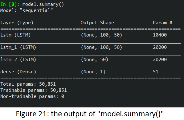
Then comes the model building. As for this stacked LSTM model (an extension of LSTM model with multiple hidden layers), I used the “Sequential” model with an additional of four layers:

model = Sequential()
model.add(LSTM(50, return_sequences = True, input_shape = (100,1)))
model.add(LSTM(50, return_sequences = True))
model.add(LSTM(50))
model.add(Dense(1))
model.compile(loss='mean_squared_error', optimizer = 'adam')

I prepared two arrays of train and test predictions data by shifting the data to be able to graph it with the actual price.
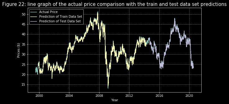
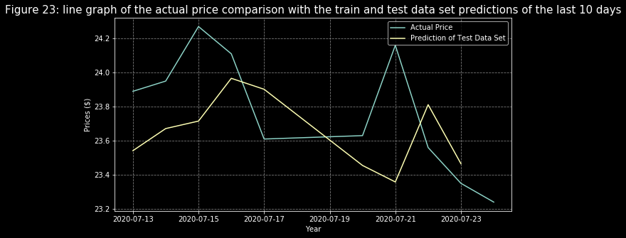
Then, I plotted the actual price, the prediction of the train data set, and the prediction of the test data set. Figure 22 showed a big picture of how good the accuracy is for the prediction is to the actual data. This means that with the current model, I could identify the general trend of the stock. Looking into it more closely with figure 23, here I only showed data of the last 10 days, it is now easier to see the precision of the prediction is not so great. There seems to be a little bit of a delay in the prediction in terms of changes that happened to the stock prices.

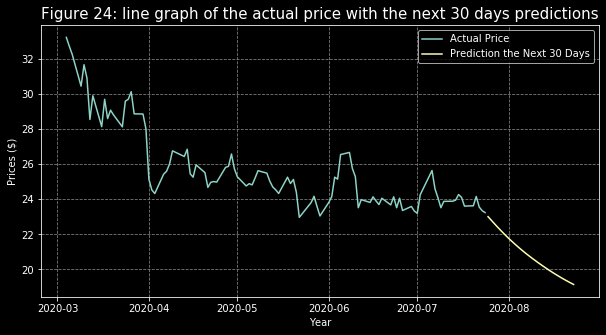
The last thing I tried to do with the project is to predict the next 30 days of the closing price of the HSBC stock. I used the code from Krish’s YouTube video to perform this prediction. The steps for preparing the data (such as reshaping) and applying the input data set into the model are very similar as I did above. The only difference for this part was adding the logic of continuing to add the new price prediction into the input data set and make it keep predicting on a loop. In the end, the output of predictions looked like the figure below.

Overall Model Performance

In the train and test data set predictions' performances, I took the prediction from the model and reshaped it back to the original form. The last step is to find the RMSE of the test and train data set by taking the square root of the “mean_squared_error” function:

.	Train Data Set	Test Data Set
Root Mean Square Error	32.3823361526875	34.503165661139754

Conclusion

Because both RMSE of train and test data set are very closed and small, I can say that the model did very well in predicting the stock prices of HSBC (especially predicting the general trend of the future prices). But taking a look at the 30 days prediction, I would not depend on it too much. I am surprised to see that the model’s prediction is opposite from mine: that the stock will go down in price. If this is true, it will be quite concerning for the bank because the stock price had not gone that low for years. Maybe the pandemic might affect the stock market in some way but I do not think that the model took the pandemic into the account here. All jokes aside, I could conclude that the further into the future the model has to guess, the less accurate and precise the prediction can be. I felt that this project would be very beneficial to those who are investors than traders. The reason being traders need precision while investors only need to know the trend of the stock price.

Overall, I believed that I did a very good job of analyzing the HSBC stock and implementing the stacked LSTM model to predict the future close price. Something I could change if I revisit this project is to try different numbers of hidden layers for the model and the layers itself to see if it can better predict the price. I could also use a different performance metric, such as mean absolute error (MAE), to determine the performance of the model.

If I were to continue this project, I would spend more time developing a stronger trading plan that involves different special candlesticks/ patterns and presented it in the EDA section. It would also be very interesting to compare different models' performances (such as stacked LSTM and a different model where I can have the candlesticks/ patterns as variables instead of only the closing price) to see whether there is any model out there that can beat a deep learning model in predicting stock prices.